Project 2 Post

Summary

This project is an EDA on Top 100 Billboard Tracks in 2000. The raw data have the following features with 317 rows

track names
artists
genre
date-entered
date-peaked
ranks by week

Hypothesis

My goal is to test two hypothesis on a 95% confidence level, which focused on the Genre column

Hypothesis 1: Country genre has has no difference with overall music in terms of number of days between the tracked entered and peaked on Billboard

Hypothesis 2: Rock genre has no difference with R&B genre in terms of the number of weeks the track stayed on Billboard

Project steps

Here are the steps I took:

Get data:

Took a quick look at the data
Identified assumptions and problems
- I found mistakes on the data entry. For example, Breathe by Faith Hill was considered as Rap, while I would consider it as pop music.
- I assumed the peaked date was when the track had the highest rank on Billboard, even if some tracks were entered before 2000.

Clean Data

Before I went further to my analysis, I spent quite an amount of time on cleaning data. As I was cleaning I revealed new problems. Over and over, the dataset became easier and nicer to work on.

Create a function to convert * to NaN and removed columns after ‘x65th.week’ because those columns only contains NaN values
Clean ‘time’, ‘date.entered’ and ‘date.peaked’ columns
- Use functions like str.replace, .strip, to_datetime.dt.time and tp_datetime
Clean week columns to float
Clean column ‘genre’
- Combine same values in different format, i.e. ‘R&B’ and ‘R & B’, ‘Rock’ and ‘Rock’n’roll’

Analyze Data

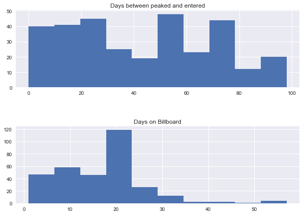
Since I was interested in the number of weeks that tracks stayed on Billboard, as well as the time difference between the tracked entered and peaked on Billboard, I created 2 new features.

Created ‘diff.between.peaked.and.enetered’ column
- Substracted ‘date.entered’ from ‘date.peaked’ and converted them into integer
Create ‘no.of.weeks.on.billboard’ column
- Used a for loop to count # of weeks
- Transformed the list into pandas series
Visualizations
- Days between entered and peaked histogram
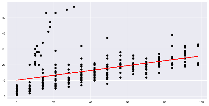
- Linear regression scatter plot

Test Results

Hypothesis 1: Country genre has has no difference with overall music in terms of number of days between the tracked entered and peaked on Billboard

P-value is much less than 0.05. so we do not accept H0. We believe there is a difference between country music and overall music in terms of number of days between the track peaked and entered

Hypothesis 2: Rock genre has no difference with R&B genre in terms of the number of weeks the track stayed on Billboard

P-value is much less than 0.05. so we do not accept H0. We believe there is a difference between R&B and Rock music in terms of Billboard length

Next Steps

In my next steps, I would like to

Fixed the data entry mistakes in order to get more accurate resutls
Built a function calculate pvalues for each pair of genre combination

Get data

import pandas as pd
import numpy as np
import matplotlib.pyplot as plt
import seaborn as sns
from scipy import stats
from sklearn.linear_model import LinearRegression
%matplotlib inline

df = pd.read_csv("assets/billboard.csv")

df.head()

	year	artist.inverted	track	time	genre	date.entered	date.peaked	x1st.week	x2nd.week	x3rd.week	...	x67th.week	x68th.week	x69th.week	x70th.week	x71st.week	x72nd.week	x73rd.week	x74th.week	x75th.week	x76th.week
0	2000	Destiny's Child	Independent Women Part I	3,38,00 AM	Rock	September 23, 2000	November 18, 2000	78	63	49	...	*	*	*	*	*	*	*	*	*	*
1	2000	Santana	Maria, Maria	4,18,00 AM	Rock	February 12, 2000	April 8, 2000	15	8	6	...	*	*	*	*	*	*	*	*	*	*
2	2000	Savage Garden	I Knew I Loved You	4,07,00 AM	Rock	October 23, 1999	January 29, 2000	71	48	43	...	*	*	*	*	*	*	*	*	*	*
3	2000	Madonna	Music	3,45,00 AM	Rock	August 12, 2000	September 16, 2000	41	23	18	...	*	*	*	*	*	*	*	*	*	*
4	2000	Aguilera, Christina	Come On Over Baby (All I Want Is You)	3,38,00 AM	Rock	August 5, 2000	October 14, 2000	57	47	45	...	*	*	*	*	*	*	*	*	*	*

5 rows × 83 columns

df.info()

<class 'pandas.core.frame.DataFrame'>
RangeIndex: 317 entries, 0 to 316
Data columns (total 83 columns):
year               317 non-null int64
artist.inverted    317 non-null object
track              317 non-null object
time               317 non-null object
genre              317 non-null object
date.entered       317 non-null object
date.peaked        317 non-null object
x1st.week          317 non-null int64
x2nd.week          317 non-null object
x3rd.week          317 non-null object
x4th.week          317 non-null object
x5th.week          317 non-null object
x6th.week          317 non-null object
x7th.week          317 non-null object
x8th.week          317 non-null object
x9th.week          317 non-null object
x10th.week         317 non-null object
x11th.week         317 non-null object
x12th.week         317 non-null object
x13th.week         317 non-null object
x14th.week         317 non-null object
x15th.week         317 non-null object
x16th.week         317 non-null object
x17th.week         317 non-null object
x18th.week         317 non-null object
x19th.week         317 non-null object
x20th.week         317 non-null object
x21st.week         317 non-null object
x22nd.week         317 non-null object
x23rd.week         317 non-null object
x24th.week         317 non-null object
x25th.week         39 non-null object
x26th.week         37 non-null object
x27th.week         30 non-null object
x28th.week         317 non-null object
x29th.week         317 non-null object
x30th.week         317 non-null object
x31st.week         317 non-null object
x32nd.week         317 non-null object
x33rd.week         317 non-null object
x34th.week         317 non-null object
x35th.week         317 non-null object
x36th.week         317 non-null object
x37th.week         317 non-null object
x38th.week         317 non-null object
x39th.week         317 non-null object
x40th.week         317 non-null object
x41st.week         317 non-null object
x42nd.week         317 non-null object
x43rd.week         317 non-null object
x44th.week         317 non-null object
x45th.week         317 non-null object
x46th.week         317 non-null object
x47th.week         317 non-null object
x48th.week         317 non-null object
x49th.week         317 non-null object
x50th.week         317 non-null object
x51st.week         317 non-null object
x52nd.week         317 non-null object
x53rd.week         317 non-null object
x54th.week         317 non-null object
x55th.week         317 non-null object
x56th.week         317 non-null object
x57th.week         317 non-null object
x58th.week         317 non-null object
x59th.week         317 non-null object
x60th.week         317 non-null object
x61st.week         317 non-null object
x62nd.week         317 non-null object
x63rd.week         317 non-null object
x64th.week         317 non-null object
x65th.week         317 non-null object
x66th.week         317 non-null object
x67th.week         317 non-null object
x68th.week         317 non-null object
x69th.week         317 non-null object
x70th.week         317 non-null object
x71st.week         317 non-null object
x72nd.week         317 non-null object
x73rd.week         317 non-null object
x74th.week         317 non-null object
x75th.week         317 non-null object
x76th.week         317 non-null object
dtypes: int64(2), object(81)
memory usage: 205.6+ KB

Clean Data

Replace * to NaN
Remove NaN value columns
Convert time column to datetime
Convert rank column to float
Clean genre column

# replace * to NaN
def _convert_nan(value):
    if value == '*':
        return np.nan
    else:
        return value
df = df.applymap(_convert_nan)

# Remove column 'year' and columns after 'x66th.week' - these columns only contains year 2000 or Nan
df= df.loc[:,'artist.inverted':'x65th.week']

# Convert time to the correct format
df['time'] = df['time'].str.replace(",",":")
df['time'] = df['time'].str.strip(' AM')

df['time'] = pd.to_datetime(df['time']).dt.time

# Convert date to datetime type
df['date.entered'] = pd.to_datetime(df['date.entered'])
df['date.peaked'] = pd.to_datetime(df['date.peaked'])

# Convert rank to float
df.loc[:,'x1st.week':'x65th.week'] = df.loc[:,'x1st.week':'x65th.week'].applymap(lambda x: float(x))

# Replace 'R & B' with 'R&B and 'Rock'n'roll' with 'Rock' due to typo
df['genre'] = df['genre'].apply(lambda x: x.replace('R & B','R&B'))
df['genre'] = df['genre'].apply(lambda x: x.replace("Rock'n'roll","Rock"))

df.info()

<class 'pandas.core.frame.DataFrame'>
RangeIndex: 317 entries, 0 to 316
Data columns (total 71 columns):
artist.inverted    317 non-null object
track              317 non-null object
time               317 non-null object
genre              317 non-null object
date.entered       317 non-null datetime64[ns]
date.peaked        317 non-null datetime64[ns]
x1st.week          317 non-null float64
x2nd.week          312 non-null float64
x3rd.week          307 non-null float64
x4th.week          300 non-null float64
x5th.week          292 non-null float64
x6th.week          280 non-null float64
x7th.week          269 non-null float64
x8th.week          260 non-null float64
x9th.week          253 non-null float64
x10th.week         244 non-null float64
x11th.week         236 non-null float64
x12th.week         222 non-null float64
x13th.week         210 non-null float64
x14th.week         204 non-null float64
x15th.week         197 non-null float64
x16th.week         182 non-null float64
x17th.week         177 non-null float64
x18th.week         166 non-null float64
x19th.week         156 non-null float64
x20th.week         146 non-null float64
x21st.week         65 non-null float64
x22nd.week         55 non-null float64
x23rd.week         48 non-null float64
x24th.week         46 non-null float64
x25th.week         38 non-null float64
x26th.week         36 non-null float64
x27th.week         29 non-null float64
x28th.week         24 non-null float64
x29th.week         20 non-null float64
x30th.week         20 non-null float64
x31st.week         19 non-null float64
x32nd.week         18 non-null float64
x33rd.week         12 non-null float64
x34th.week         10 non-null float64
x35th.week         9 non-null float64
x36th.week         9 non-null float64
x37th.week         9 non-null float64
x38th.week         8 non-null float64
x39th.week         8 non-null float64
x40th.week         7 non-null float64
x41st.week         7 non-null float64
x42nd.week         6 non-null float64
x43rd.week         6 non-null float64
x44th.week         6 non-null float64
x45th.week         5 non-null float64
x46th.week         5 non-null float64
x47th.week         5 non-null float64
x48th.week         4 non-null float64
x49th.week         4 non-null float64
x50th.week         4 non-null float64
x51st.week         4 non-null float64
x52nd.week         4 non-null float64
x53rd.week         4 non-null float64
x54th.week         2 non-null float64
x55th.week         2 non-null float64
x56th.week         2 non-null float64
x57th.week         2 non-null float64
x58th.week         2 non-null float64
x59th.week         2 non-null float64
x60th.week         2 non-null float64
x61st.week         2 non-null float64
x62nd.week         2 non-null float64
x63rd.week         2 non-null float64
x64th.week         2 non-null float64
x65th.week         1 non-null float64
dtypes: datetime64[ns](2), float64(65), object(4)
memory usage: 175.9+ KB

Analysis

Create new columns ‘diff. between date peaked and entered’ and ‘no. of weeks on billboard’
Create histograms for new columns
Create scatter plot for ‘diff. between date peaked and entered’ and ‘no. of weeks on billboard’
Pivot table on ‘genre’

# Create a new column of diff. between date peaked and entered
df['diff.between.peaked.and.enetered'] = (df['date.peaked']-df['date.entered']).astype(str)

# Convert the column to integer
df['diff.between.peaked.and.enetered'] = df['diff.between.peaked.and.enetered'].apply(lambda x: int(x[0:2]))

# Create a column for no. of weeks on billboard
# Slice data into Week on billboard only
week_df = df.loc[:,'x1st.week':'x65th.week']

# Create a list of no. of weeks on billboard for each song
# Add the column to the dataframe
no_week_list=[]
for i in range(len(week_df)):
    no_week_list.append(week_df.iloc[i,:].count())
df['no.of.weeks.on.billboard'] = pd.Series(no_week_list)

# Create histograms for new columns
fig, axes = plt.subplots(2,1, figsize = (10,7))
fig.subplots_adjust(wspace = 0.25, hspace = 0.5)

axes[0].hist(df['diff.between.peaked.and.enetered'])
axes[0].set_title('Days between peaked and entered')
axes[1].hist(df['no.of.weeks.on.billboard'])
axes[1].set_title('Days on Billboard');

png

# Create scatter plot and regression for 'diff. between date peaked and entered' and 'no. of weeks on billboard'

regr = LinearRegression()
X = df[['diff.between.peaked.and.enetered']]
y = df['no.of.weeks.on.billboard']
model = regr.fit(X,y)

fig, ax = plt.subplots(figsize=(12,6))

ax.scatter(X,y,c='k')
ax.plot(X,regr.predict(X),color='r');
print model.score(X,y)

/Users/KatieJi/anaconda/lib/python2.7/site-packages/scipy/linalg/basic.py:1018: RuntimeWarning: internal gelsd driver lwork query error, required iwork dimension not returned. This is likely the result of LAPACK bug 0038, fixed in LAPACK 3.2.2 (released July 21, 2010). Falling back to 'gelss' driver.
  warnings.warn(mesg, RuntimeWarning)


0.220245120868

png

df.head()

	artist.inverted	track	time	genre	date.entered	date.peaked	x1st.week	x2nd.week	x3rd.week	x4th.week	...	x58th.week	x59th.week	x60th.week	x61st.week	x62nd.week	x63rd.week	x64th.week	x65th.week	diff.between.peaked.and.enetered	no.of.weeks.on.billboard
0	Destiny's Child	Independent Women Part I	03:38:00	Rock	2000-09-23	2000-11-18	78.0	63.0	49.0	33.0	...	NaN	NaN	NaN	NaN	NaN	NaN	NaN	NaN	56	28
1	Santana	Maria, Maria	04:18:00	Rock	2000-02-12	2000-04-08	15.0	8.0	6.0	5.0	...	NaN	NaN	NaN	NaN	NaN	NaN	NaN	NaN	56	26
2	Savage Garden	I Knew I Loved You	04:07:00	Rock	1999-10-23	2000-01-29	71.0	48.0	43.0	31.0	...	NaN	NaN	NaN	NaN	NaN	NaN	NaN	NaN	98	33
3	Madonna	Music	03:45:00	Rock	2000-08-12	2000-09-16	41.0	23.0	18.0	14.0	...	NaN	NaN	NaN	NaN	NaN	NaN	NaN	NaN	35	24
4	Aguilera, Christina	Come On Over Baby (All I Want Is You)	03:38:00	Rock	2000-08-05	2000-10-14	57.0	47.0	45.0	29.0	...	NaN	NaN	NaN	NaN	NaN	NaN	NaN	NaN	70	21

5 rows × 73 columns

# See value counts on 'genre'
df['genre'].value_counts()

Rock           137
Country         74
Rap             58
R&B             23
Pop              9
Latin            9
Electronica      4
Gospel           1
Jazz             1
Reggae           1
Name: genre, dtype: int64

# Pivot table on genre
pd.pivot_table(df,index = 'genre', values = ['diff.between.peaked.and.enetered','no.of.weeks.on.billboard'],aggfunc = (np.mean, np.std))

	diff.between.peaked.and.enetered		no.of.weeks.on.billboard
	mean	std	mean	std
genre
Country	52.472973	25.048568	16.216216	7.270263
Electronica	61.250000	10.500000	18.000000	4.000000
Gospel	56.000000	NaN	20.000000	NaN
Jazz	14.000000	NaN	5.000000	NaN
Latin	51.222222	32.976423	19.222222	7.293452
Pop	47.444444	25.666667	15.222222	8.120618
R&B	28.608696	24.332431	11.347826	6.176265
Rap	34.862069	24.914907	14.431034	8.764186
Reggae	42.000000	NaN	15.000000	NaN
Rock	41.343066	28.954436	18.883212	10.195202

Evaluate Statements

Statement 1: Country music has no difference with overall music in terms of the no. of days between peaked and entered
H0: country musice mean = overall mean H1: country musice mean != overall mean
Statement 2: Rock music has no difference with R&B music in terms of the no. of weeks on billboard
H0: rock musice mean = R&B music mean H1: rock musice mean > R&B music mean

# Statement 1 Test, set alpha = 0.05
print stats.ttest_1samp(df[df['genre']=='Country']['diff.between.peaked.and.enetered'],overall_mean)

Ttest_1sampResult(statistic=3.4255181858814843, pvalue=0.0010106239460667809)

Pvalue is less than 0.05. We do not accept H0. There is a difference between country music and overall music in terms of no. of days between peaked and entered

# Statement 2 Test, set aplha = 0.05
print stats.ttest_ind(df[df['genre']=='Rock']['no.of.weeks.on.billboard'],df[df['genre']=='R&B']['no.of.weeks.on.billboard'])

Ttest_indResult(statistic=3.4348656996446518, pvalue=0.00075739756196112828)

Pvalue is less than 0.05. We do not accept H0. Rock music siganificantly stays longer than R&B music on billboard

Written on April 4, 2017