
Project 6
Movie Ratings Project
In this project, I used classification modeling to examine what factors lead to certain ratings for movies, based on a dataset I collected from IMDB (www.imdb.com).
Assumption
Before we go to the results, here are two major assumptions I made for this project.
- Data collection: data was collected from two parts
- Top 250 movies on IMDB
- The 50 most popular movies by genre (action, adventure, animation, biography, comedy, crime, documentary, drama, family, fantasy, history, horror, musical, mystery, romance, sport, thriller, war, western).
- Labeling: imdb rating is my dependent variable. The lowest imdb rating for the top 250 movies was 8.0. I labeled
- 1 for movies that had imdb rating equal or above 8.0
- 0 for movies that had imdb rating below 8.0
- Imputing: imputed means for NaN values in Box office and Metascore columns
Summary
I applied Random forest and Extra trees for the modeling section. Both models had the number of imdbvotes, movie year and Metascore in the top 5 features.
A greater number of imdbvotes indicates more people have watched the movie. This can a factor to see if the movie is sucessful or not.
Old movies are more likely to be rated higher. Since I collected the data from the best and the most popular movies, old movies that are still popular are usually classic and great ones.
Metascore has a relatively positive relationship with imdbrating. That means it contains some information for my dependent variable.
Random forests had a higher accuracy score on test dataset (0.78 vs 0.72)
Project Outline
- Get data
- Clean data
- Add features
- Visualization
- Random Forest
- Extra trees
Next Steps
In next steps, I would like to take a deeper look around my assumptions.
- Data collection: get a list of randomly selected movies since 1900 and webscrape more data
- Apply KNN imputer for NaN values
- Examine outliners in visualizations
- Try more models eg. baggings, boosting, logistic regression.
import requests
import pandas as pd
from imdbpie import Imdb
import numpy as np
Get data
# Get top250 movies from imdbpie
imdb = Imdb()
imdb = Imdb(anonymize=True)
top_250 = imdb.top_250()
df_top_250 = pd.DataFrame(top_250)
df_top_250.head()
| can_rate | image | num_votes | rating | tconst | title | type | year | |
|---|---|---|---|---|---|---|---|---|
| 0 | True | {u'url': u'https://images-na.ssl-images-amazon... | 1808376 | 9.3 | tt0111161 | The Shawshank Redemption | feature | 1994 |
| 1 | True | {u'url': u'https://images-na.ssl-images-amazon... | 1234863 | 9.2 | tt0068646 | The Godfather | feature | 1972 |
| 2 | True | {u'url': u'https://images-na.ssl-images-amazon... | 849748 | 9.0 | tt0071562 | The Godfather: Part II | feature | 1974 |
| 3 | True | {u'url': u'https://images-na.ssl-images-amazon... | 1788444 | 9.0 | tt0468569 | The Dark Knight | feature | 2008 |
| 4 | True | {u'url': u'https://images-na.ssl-images-amazon... | 489687 | 8.9 | tt0050083 | 12 Angry Men | feature | 1957 |
id_list_1 = df_top_250['tconst'].tolist()
# Get 50 popular movies for each genre
import requests
from bs4 import BeautifulSoup
genre = ['action','adventure','animation','biography','comedy','crime', 'documentary','drama','family', 'fantasy'\
         ,'history', 'horror', 'musical', 'mystery', 'romance','sport','thriller','war', 'western']
id_list_2 = []

for i in genre:
    url = 'http://www.imdb.com/search/title?genres={}&title_type=feature&sort=moviemeter,asc&page=1&ref_=adv_nxt'.format(i)
    r = requests.get(url)
    soup = BeautifulSoup(r.content,'lxml')
    div = soup.findAll('div',class_='ribbonize')
    for k in div:
        id_number = k.get('data-tconst')
        id_list_2.append(id_number)
len(id_list_2)
900
id_list = id_list_1 + id_list_2
len(id_list)
1150
# Search imdb ID on omdbapi

df_origin = pd.DataFrame()

for i in id_list:
    r = requests.get('http://www.omdbapi.com/?i={}&plot=short&r=json'.format(i))
    df_i=pd.DataFrame(r.json())
    df_origin = df_origin.append(df_i)
Clean data
1. Drop duplicates
df = df_origin.drop_duplicates(subset =['imdbID'], keep='first').reset_index(drop=True)
2. Drop columns
df.columns
Index([u'Actors', u'Awards', u'BoxOffice', u'Country', u'DVD', u'Director',
       u'Genre', u'Language', u'Metascore', u'Plot', u'Poster', u'Production',
       u'Rated', u'Ratings', u'Released', u'Response', u'Runtime', u'Title',
       u'Type', u'Website', u'Writer', u'Year', u'imdbID', u'imdbRating',
       u'imdbVotes'],
      dtype='object')
df = df.drop(['Poster','Website','Type','Response','Ratings','Production'],axis=1)
3. Replace ‘N/A’ with NaN
df = df.replace('N/A',np.nan)
df = df.dropna(subset=['imdbRating'])
4. Clean Country, Genre and Language
def clean_orders(column_name):
    df[column_name] = df[column_name].apply(lambda x: x.split(', '))
    df[column_name] = df[column_name].apply(lambda x: sorted(x))
    df[column_name] = df[column_name].apply(lambda x: ', '.join(x))
clean_orders('Country')
clean_orders('Genre')
df['Language'][df['Language'].isnull()] ='English'
clean_orders('Language')
5. Clean Runtime, Year, imdbRating and imdbVotes
df['Runtime'][df['Runtime'].isnull()] = '91 min'
df['Runtime'] = df['Runtime'].apply(lambda x: int(str(x).strip(' min')))
df['Year'] = df['Year'].apply(lambda x: int(x))
df['imdbRating'] = df['imdbRating'].apply(lambda x: float(x))
df['imdbVotes'] = df['imdbVotes'].apply(lambda x: x.replace(',',''))
df['imdbVotes'] = df['imdbVotes'].apply(lambda x: int(x))
6. Clean DVD and Released dates
df['DVD'] = pd.to_datetime(df['DVD'])
df['Released'] = pd.to_datetime(df['Released'])
df['DVD'].fillna(df['Year'],inplace=True)
df['Released'].fillna(df['Year'],inplace=True)
7. Clean Rated
df['Rated'] = df['Rated'].apply(lambda x: str(x).replace('NOT RATED','UNRATED'))
df['Rated'] = df['Rated'].apply(lambda x: str(x).replace('PASSED','APPROVED'))
df['Rated'] = df['Rated'].apply(lambda x: str(x).replace('nan','UNRATED'))
8. Clean Awards
df['Nominations']= df['Awards'].str.extract('([0-9]+ nominations)')
/Users/KatieJi/anaconda/lib/python2.7/site-packages/ipykernel/__main__.py:1: FutureWarning: currently extract(expand=None) means expand=False (return Index/Series/DataFrame) but in a future version of pandas this will be changed to expand=True (return DataFrame)
  if __name__ == '__main__':
df['Nominations'] = df['Nominations'].apply(lambda x: float(str(x).replace(' nominations','')))
df['Nominations'] = df['Nominations'].fillna(0)
df['Wins']= df['Awards'].str.extract('([0-9]+ wins)')
/Users/KatieJi/anaconda/lib/python2.7/site-packages/ipykernel/__main__.py:1: FutureWarning: currently extract(expand=None) means expand=False (return Index/Series/DataFrame) but in a future version of pandas this will be changed to expand=True (return DataFrame)
  if __name__ == '__main__':
df['Wins'] = df['Wins'].apply(lambda x: float(str(x).replace(' wins','')))
df['Wins'] = df['Wins'].fillna(0)
df['Oscars']= df['Awards'].str.extract('([0-9]+ Oscars)')
/Users/KatieJi/anaconda/lib/python2.7/site-packages/ipykernel/__main__.py:1: FutureWarning: currently extract(expand=None) means expand=False (return Index/Series/DataFrame) but in a future version of pandas this will be changed to expand=True (return DataFrame)
  if __name__ == '__main__':
df['Oscars'] = df['Oscars'].apply(lambda x: float(str(x).replace(' Oscars','')))
df['Oscars'] = df['Oscars'].fillna(0)
df = df.drop(['Awards'],axis=1)
df['BoxOffice']=df['BoxOffice'].apply(lambda x: str(x).replace('$',''))
df['BoxOffice']=df['BoxOffice'].apply(lambda x: str(x).replace(',',''))
df['BoxOffice']=df['BoxOffice'].apply(lambda x: str(x).replace('.',''))
df['BoxOffice']=df['BoxOffice'].apply(lambda x: float(x)/100)
df['Metascore']=df['Metascore'].apply(lambda x: float(x))
df.head(3)
| Actors | BoxOffice | Country | DVD | Director | Genre | Language | Metascore | Plot | Rated | ... | Labels | rated__APPROVED | rated__G | rated__GP | rated__PG | rated__PG-13 | rated__R | rated__TV-14 | rated__TV-MA | rated__UNRATED | |
|---|---|---|---|---|---|---|---|---|---|---|---|---|---|---|---|---|---|---|---|---|---|
| 0 | Tim Robbins, Morgan Freeman, Bob Gunton, Willi... | NaN | USA | 1970-01-01 00:00:00.000001994 | Frank Darabont | Crime, Drama | English | 80.0 | Two imprisoned men bond over a number of years... | R | ... | 1 | 0 | 0 | 0 | 0 | 0 | 1 | 0 | 0 | 0 |
| 1 | Marlon Brando, Al Pacino, James Caan, Richard ... | NaN | USA | 2001-10-09 00:00:00.000000000 | Francis Ford Coppola | Crime, Drama | English, Italian, Latin | 100.0 | The aging patriarch of an organized crime dyna... | R | ... | 1 | 0 | 0 | 0 | 0 | 0 | 1 | 0 | 0 | 0 |
| 2 | Al Pacino, Robert Duvall, Diane Keaton, Robert... | NaN | USA | 1970-01-01 00:00:00.000001974 | Francis Ford Coppola | Crime, Drama | English, Italian, Latin, Sicilian, Spanish | 80.0 | The early life and career of Vito Corleone in ... | R | ... | 1 | 0 | 0 | 0 | 0 | 0 | 1 | 0 | 0 | 0 |
3 rows × 32 columns
df_clean = df
df = df_clean
Adding Features
1. Add a new feature Age
df['Age'] = 2017 - df['Year']
2. Label y based on imdb ratings
# top 250 movies have ratings greater than 8 - consider ratings greater than 8 as high ratings
df['Labels'] = df['imdbRating'].apply(lambda x: 1 if x >= 8.0 else 0)
df_high = df[df['Labels']==1]
df_low = df[df['Labels']==0]
Visualization
import matplotlib.pyplot as plt
import seaborn as sns
%matplotlib inline
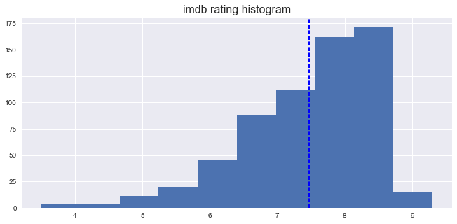
1. Histogram on imdb ratings
From the imdbratings histogram, these movies have a mean of ratings about 7.5.
Most of the ratings are around 6-8.5
fig = plt.figure(figsize=(11,5))
df['imdbRating'].hist()
plt.axvline(df['imdbRating'].mean(),color='b', linestyle='dashed', linewidth=2)
plt.title('imdb rating histogram',fontsize = 16)
<matplotlib.text.Text at 0x111ee2710>
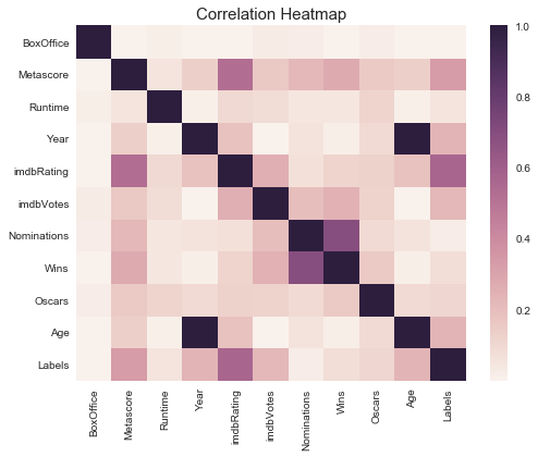
2. Heatmap
Age and Year have a very strong relationship because I calculated Age by deducting year from 2017
Wins and Nominations also have a strong relationship, so do Metascore and imdbrating
fig=plt.figure(figsize=(8,6))
sns.heatmap(df.corr()**2)
plt.title('Correlation Heatmap', fontsize=15);
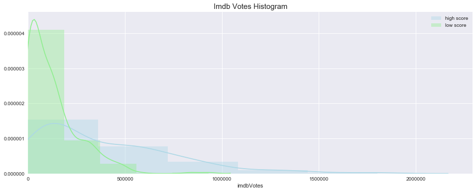
3. imdbvotes histogram
I plotted imdb votes by type (high score or low score).
It looks like the low-scored movies are more likely to have fewer votes.
high-scored movies are more widely distributed compared to low-scored movies
df_high.columns
Index([     u'Actors',   u'BoxOffice',     u'Country',         u'DVD',
          u'Director',       u'Genre',    u'Language',   u'Metascore',
              u'Plot',       u'Rated',    u'Released',     u'Runtime',
             u'Title',      u'Writer',        u'Year',      u'imdbID',
        u'imdbRating',   u'imdbVotes', u'Nominations',        u'Wins',
            u'Oscars',         u'Age',      u'Labels'],
      dtype='object')
fig = plt.figure(figsize=(16,6))
sns.distplot(df_high['imdbVotes'],color='lightblue',label='high score',bins=5)
sns.distplot(df_low['imdbVotes'],color='lightgreen',label='low score',bins=5)
plt.xlim(0)
plt.title('Imdb Votes Histogram', fontsize=15)
plt.legend();
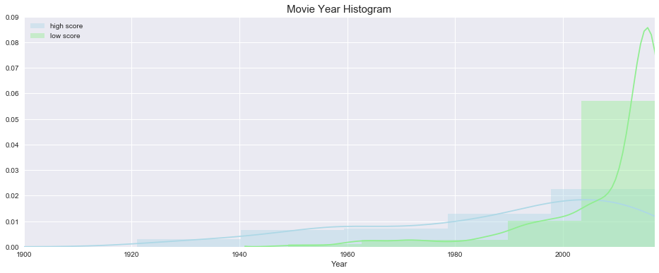
4. Year histogram
Low-scored movies are more likely to be recent movies after 2000
High-scored movies are more evenly distributed through 1920 - 2017, while the amount of movies have been increasing through years
fig = plt.figure(figsize=(16,6))
sns.distplot(df_high['Year'],color='lightblue',label='high score',bins=5)
sns.distplot(df_low['Year'],color='lightgreen',label='low score',bins=5)
plt.xlim(1900,2017)
plt.title('Movie Year Histogram', fontsize=15)
plt.legend();
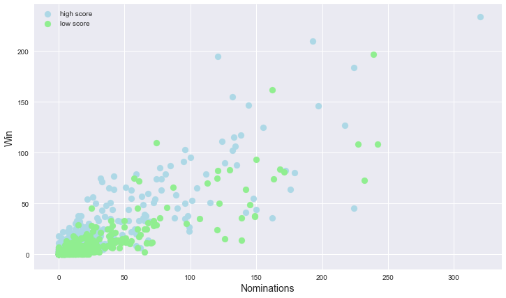
5. Scatter for Nominations and Wins
From the graph, it looks like Nominations and Wins have a positive linear relationship.
High-scored movies have a higher chance to get above 50 wins and 50 nominations.
mask_high= df_high[df_high['Year']!=2017]
mask_low= df_low[df_low['Year']!=2017]
fig = plt.figure(figsize=(12,7))
ax = fig.gca()
plt.scatter(mask_high['Nominations'],mask_high['Wins'],c='lightblue',s=80)
plt.scatter(mask_low['Nominations'],mask_low['Wins'],c='lightgreen',s=80)

ax.set_xlabel('Nominations',fontsize=14)
ax.set_ylabel('Win',fontsize=14)

plt.legend(['high score', 'low score']);
Feature engineering
1. Get dummy variables for rated
df= df.join(pd.get_dummies(df['Rated'],prefix='rated_'))
2. Train Test split
from sklearn.model_selection import train_test_split
X = df.drop(['imdbRating','imdbID','Labels', 'Rated','DVD','Released'],axis=1)
y = df['Labels']

X_train, X_test, y_train, y_test = train_test_split(X, y, stratify=y, random_state = 42, test_size=.33)
X_train.reset_index(drop=True, inplace=True)
X_test.reset_index(drop=True, inplace=True)

y_train.reset_index(drop=True, inplace=True)
y_test.reset_index(drop=True, inplace=True)
X_train.head(3)
| Actors | BoxOffice | Country | Director | Genre | Language | Metascore | Plot | Runtime | Title | ... | Age | rated__APPROVED | rated__G | rated__GP | rated__PG | rated__PG-13 | rated__R | rated__TV-14 | rated__TV-MA | rated__UNRATED | |
|---|---|---|---|---|---|---|---|---|---|---|---|---|---|---|---|---|---|---|---|---|---|
| 0 | Mia Goth, Martin McCann, Andrew Simpson, Barry... | NaN | UK | Stephen Fingleton | Drama, Sci-Fi, Thriller | English | NaN | In a time of starvation, a survivalist lives o... | 104 | The Survivalist | ... | 2 | 0 | 0 | 0 | 0 | 0 | 0 | 0 | 0 | 1 |
| 1 | Charlie Hunnam, Sienna Miller, Tom Holland, Ro... | 66320.68 | USA | James Gray | Action, Adventure, Biography | English, German, Portuguese, Spanish | 84.0 | A true-life drama, centering on British explor... | 141 | The Lost City of Z | ... | 1 | 0 | 0 | 0 | 0 | 1 | 0 | 0 | 0 | 0 |
| 2 | Charles Chaplin, Paulette Goddard, Henry Bergm... | NaN | USA | Charles Chaplin | Comedy, Drama, Family | English | 96.0 | The Tramp struggles to live in modern industri... | 87 | Modern Times | ... | 81 | 0 | 1 | 0 | 0 | 0 | 0 | 0 | 0 | 0 |
3 rows × 26 columns
3. Create dummy variables using NLP
from sklearn.feature_extraction.text import CountVectorizer
def cvec(df,columns,n_range,max_f):
    cvec = CountVectorizer(ngram_range=n_range,max_features=max_f)
    cvec.fit(df[columns])
    return pd.DataFrame(cvec.transform(df[columns]).todense(),
             columns=cvec.get_feature_names())
actors = cvec(X_train,'Actors',(2,3),20)
country = cvec(X_train,'Country',(1,1),20)
genre = cvec(X_train,'Genre',(1,1),20)
language = cvec(X_train,'Language',(1,1),20)
writer = cvec(X_train,'Writer',(2,3),20)
title = cvec(X_train,'Title',(1,1),20)
director = cvec(X_train,'Director',(2,3),20)
cvec = CountVectorizer(ngram_range=(1,1),max_features=20,stop_words='english')
cvec.fit(X_train['Plot'])
plot = pd.DataFrame(cvec.transform(X_train['Plot']).todense(),
         columns=cvec.get_feature_names())
dict_join = {'actors':actors, 'country': country, 'genre': genre, \
             'language': language, 'title': title, 'writer': writer, 'director':director, 'plot': plot}
for k in dict_join:
    X_train = X_train.join(dict_join[k],rsuffix=('_'+k))
from sklearn.feature_extraction.text import CountVectorizer
def cvec(df,columns,n_range,max_f):
    cvec = CountVectorizer(ngram_range=n_range,max_features=max_f)
    cvec.fit(df[columns])
    return pd.DataFrame(cvec.transform(df[columns]).todense(),
             columns=cvec.get_feature_names())
actors_test = cvec(X_test,'Actors',(2,3),20)
country_test = cvec(X_test,'Country',(1,1),20)
genre_test = cvec(X_test,'Genre',(1,1),20)
language_test = cvec(X_test,'Language',(1,1),20)
writer_test = cvec(X_test,'Writer',(2,3),20)
title_test = cvec(X_test,'Title',(1,1),20)
director_test = cvec(X_test,'Director',(2,3),20)
cvec = CountVectorizer(ngram_range=(1,1),max_features=20,stop_words='english')
cvec.fit(X_test['Plot'])
plot_test = pd.DataFrame(cvec.transform(X_test['Plot']).todense(),
         columns=cvec.get_feature_names())
dict_join_test = {'actors':actors_test, 'country': country_test, 'genre': genre_test, \
             'language': language_test, 'title': title_test, 'writer': writer_test, \
                  'director':director_test, 'plot': plot_test}
for k in dict_join_test:
    X_test = X_test.join(dict_join_test[k],rsuffix=('_'+k))
X_train = X_train.drop(['Actors','Country','Director','Genre','Language','Plot','Title','Writer','Year'],axis=1)
X_test = X_test.drop(['Actors','Country','Director','Genre','Language','Plot','Title','Writer','Year'],axis=1)
4. Impute mean for Boxoffice and Metascore
from sklearn.preprocessing import Imputer

imputer_m = Imputer(strategy='mean',axis=0).fit(X_train[['Metascore']])
imputer_b = Imputer(strategy='mean',axis=0).fit(X_train[['BoxOffice']])
X_train['Metascore'] = imputer_m.transform(X_train[['Metascore']])
X_test['Metascore'] = imputer_m.transform(X_test[['Metascore']])
X_train['BoxOffice'] = imputer_b.transform(X_train[['BoxOffice']])
X_test['BoxOffice'] = imputer_b.transform(X_test[['BoxOffice']])
5. Scaler
X_train[X_train.isnull().any(axis=1)]
| BoxOffice | Metascore | Runtime | imdbVotes | Nominations | Wins | Oscars | Age | rated__APPROVED | rated__G | ... | original story | original story by | screen story | screenplay by | story by | story development | story material | the book | the novel | the novel by |
|---|
0 rows × 177 columns
X_test[X_test.isnull().any(axis=1)]
| BoxOffice | Metascore | Runtime | imdbVotes | Nominations | Wins | Oscars | Age | rated__APPROVED | rated__G | ... | on the | on the novel | original story | original story by | screen story | screenplay christopher | stanley kubrick_writer | story by | story material | the novel |
|---|
0 rows × 177 columns
from sklearn.preprocessing import StandardScaler
scaler = StandardScaler()
scaler = scaler.fit(X_train)
X_train_s = scaler.transform(X_train)
X_test_s = scaler.transform(X_test)
Random Forest
from sklearn.tree import DecisionTreeClassifier
from sklearn.model_selection import cross_val_score, StratifiedKFold, GridSearchCV
from sklearn.ensemble import RandomForestClassifier, ExtraTreesClassifier, BaggingClassifier

from sklearn.metrics import accuracy_score, classification_report, confusion_matrix
cv = StratifiedKFold(n_splits=5 , shuffle = True, random_state = 0)

for i in [1,2,3,4,5,None]:
    print 'max depth: {}'.format(i)
    clf = DecisionTreeClassifier(max_depth=i)
    print "DT Score:\t", cross_val_score(clf, X_train_s, y_train, cv=cv, n_jobs=1).mean()
max depth: 1
DT Score:	0.700420168067
max depth: 2
DT Score:	0.763977591036
max depth: 3
DT Score:	0.830140056022
max depth: 4
DT Score:	0.851484593838
max depth: 5
DT Score:	0.849103641457
max depth: None
DT Score:	0.825518207283
grid = {
    'n_estimators': [10, 20, 30, 50, 100],
    'max_features': [1,2,3,4,5,6,'auto'],
    'criterion': ['gini','entropy'],
    'class_weight': ["balanced","balanced_subsample",None]
}

cv = StratifiedKFold(n_splits=5 , shuffle = True, random_state = 0)


clf = DecisionTreeClassifier(max_depth=4)
rf = RandomForestClassifier(clf)
gs = GridSearchCV(rf, grid)

model_rf_gs = gs.fit(X_train_s, y_train)
gs.best_params_
{'class_weight': None,
 'criterion': 'entropy',
 'max_features': 'auto',
 'n_estimators': 100}
rf = RandomForestClassifier(max_depth=4, max_features=gs.best_params_['max_features'], n_estimators=gs.best_params_['n_estimators'],\
                            criterion=gs.best_params_['criterion'],class_weight=gs.best_params_['class_weight'])
model_rf = rf.fit(X_train_s, y_train)
y_pred_train = model_rf.predict(X_train_s)
y_pred_test = model_rf.predict(X_test_s)

# Confusion matrix on test data
pd.DataFrame(confusion_matrix(y_test,y_pred_test,labels=[1,0]),\
            columns=['predicted_high','predicted_low'], index=['is_high','is_low'])
| predicted_high | predicted_low | |
|---|---|---|
| is_high | 87 | 4 |
| is_low | 41 | 77 |
# Accuracy score
print 'accuracy score on training data:', accuracy_score(y_train,y_pred_train)
print 'accuracy score on test data:', accuracy_score(y_test,y_pred_test)
accuracy score on training data: 0.929245283019
accuracy score on test data: 0.784688995215
# Get features Gini scores
feature_importances = pd.DataFrame(model_rf.feature_importances_,
                                   index = X_train.columns, columns=['importance'])
feature_importances[feature_importances['importance']!=0].sort_values(by='importance', ascending=False)
| importance | |
|---|---|
| imdbVotes | 0.163171 |
| Metascore | 0.130159 |
| Age | 0.113337 |
| Wins | 0.088582 |
| english | 0.063368 |
| Oscars | 0.035528 |
| Runtime | 0.027717 |
| Nominations | 0.027712 |
| usa | 0.023858 |
| BoxOffice | 0.022196 |
| italian | 0.015489 |
| rated__PG-13 | 0.014189 |
| italy | 0.013644 |
| musical | 0.013157 |
| hindi | 0.010673 |
| sport | 0.010616 |
| canada | 0.009466 |
| alfred hitchcock | 0.008164 |
| based on | 0.007927 |
| for | 0.006920 |
| rated__APPROVED | 0.006887 |
| horror | 0.006730 |
| comedy | 0.006597 |
| based on the | 0.005929 |
| on the | 0.005812 |
| rated__UNRATED | 0.005732 |
| french | 0.005157 |
| adventure | 0.004849 |
| war | 0.004746 |
| harrison ford | 0.004523 |
| ... | ... |
| new | 0.000495 |
| ethan coen | 0.000493 |
| arabic | 0.000490 |
| joel coen | 0.000485 |
| man | 0.000478 |
| created by | 0.000455 |
| with | 0.000451 |
| latin | 0.000448 |
| cantonese | 0.000448 |
| in | 0.000410 |
| tom hardy | 0.000399 |
| sweden | 0.000389 |
| american | 0.000370 |
| on | 0.000358 |
| to | 0.000354 |
| quentin tarantino | 0.000313 |
| additional story | 0.000304 |
| chris pratt | 0.000294 |
| ben affleck | 0.000273 |
| life | 0.000243 |
| street | 0.000196 |
| story material | 0.000194 |
| germany | 0.000180 |
| chinese | 0.000176 |
| story | 0.000159 |
| original story | 0.000147 |
| matthew mcconaughey | 0.000129 |
| book by | 0.000063 |
| johnny depp | 0.000059 |
| francis ford | 0.000014 |
140 rows × 1 columns
Extra trees
grid = {
    'n_estimators': [10, 20, 30, 50, 100],
    'max_features': [1,2,3,4,5,6,'auto'],
    'criterion': ['gini','entropy'],
    'class_weight': ["balanced", "balanced_subsample"]
}

cv = StratifiedKFold(n_splits=5 , shuffle = True, random_state = 0)


clf = DecisionTreeClassifier(max_depth=4)
et = ExtraTreesClassifier(clf,n_jobs=1)
gs_es = GridSearchCV(et, grid)

model_et_gs = gs_es.fit(X_train_s, y_train)
gs_es.best_params_
{'class_weight': 'balanced',
 'criterion': 'entropy',
 'max_features': 'auto',
 'n_estimators': 100}
es = ExtraTreesClassifier(max_depth=4, max_features=gs_es.best_params_['max_features'], n_estimators=gs_es.best_params_['n_estimators'],\
                            criterion=gs_es.best_params_['criterion'],class_weight=gs_es.best_params_['class_weight'])
model_es = es.fit(X_train_s, y_train)
y_pred_train = model_es.predict(X_train_s)
y_pred_test = model_es.predict(X_test_s)

# Confusion matrix on test data
pd.DataFrame(confusion_matrix(y_test,y_pred_test,labels=[1,0]),\
            columns=['predicted_high','predicted_low'], index=['is_high','is_low'])
| predicted_high | predicted_low | |
|---|---|---|
| is_high | 86 | 5 |
| is_low | 53 | 65 |
# Accuracy score
print 'accuracy score on training data:', accuracy_score(y_train,y_pred_train)
print 'accuracy score on test data:', accuracy_score(y_test,y_pred_test)
accuracy score on training data: 0.926886792453
accuracy score on test data: 0.722488038278
# Get features Gini scores
feature_importances = pd.DataFrame(model_es.feature_importances_,
                                   index = X_train.columns, columns=['importance'])
feature_importances[feature_importances['importance']!=0].sort_values(by='importance', ascending=False)
| importance | |
|---|---|
| Age | 0.108544 |
| Metascore | 0.079075 |
| usa | 0.074534 |
| imdbVotes | 0.070593 |
| Oscars | 0.063962 |
| english | 0.055273 |
| rated__PG-13 | 0.045749 |
| musical | 0.036524 |
| italy | 0.033469 |
| canada | 0.028664 |
| Wins | 0.023811 |
| italian | 0.023613 |
| hindi | 0.023553 |
| comedy | 0.021585 |
| harrison ford | 0.017797 |
| horror | 0.015362 |
| alfred hitchcock | 0.014934 |
| sport | 0.014587 |
| rated__UNRATED | 0.011067 |
| based on the | 0.011026 |
| rated__APPROVED | 0.009953 |
| christopher nolan | 0.009481 |
| Nominations | 0.008576 |
| sergio leone | 0.008012 |
| based on | 0.007023 |
| french | 0.006956 |
| uk | 0.006466 |
| Runtime | 0.006441 |
| family_genre | 0.006251 |
| the | 0.005942 |
| ... | ... |
| wife | 0.000550 |
| australia | 0.000543 |
| clint eastwood | 0.000542 |
| john huston | 0.000529 |
| help | 0.000528 |
| rated__PG | 0.000509 |
| tom hardy | 0.000473 |
| wars | 0.000453 |
| ben affleck | 0.000439 |
| son | 0.000433 |
| joel coen | 0.000428 |
| ewan mcgregor | 0.000413 |
| star | 0.000402 |
| life | 0.000381 |
| john musker | 0.000373 |
| animation | 0.000358 |
| back | 0.000355 |
| the book | 0.000336 |
| hungarian | 0.000321 |
| the novel | 0.000255 |
| cantonese | 0.000243 |
| ridley scott | 0.000226 |
| tom hanks | 0.000193 |
| natalie portman | 0.000192 |
| tim burton | 0.000191 |
| thriller | 0.000187 |
| germany | 0.000154 |
| gaelic | 0.000135 |
| biography | 0.000117 |
| novel by | 0.000035 |
134 rows × 1 columns